Bringing Data to Asynchronous Computing at Scale

Asynchronous computing and data processing are building blocks in the modern cloud.

The Async Tier is Meta’s platform for serverless asynchronous computing. It’s used by different engineering teams at Meta for executing arbitrary functions on a fleet of more than 100,000 workers providing capabilities such as load balancing, rate limiting, quota management, downstream protection, delayed execution, and many others. You can read more about the platform in this recently published paper.

In addition to initially supporting scheduling functions through an SDK, we’ve built first-class support for integrating arbitrary data sources within Meta, including data streams, data warehouse, and pub-sub queues. Our complete journey is described in this dedicated blog post.

The platform currently serves thousands of use cases executing more than 10 trillion jobs per day, including Near-real-time Abuse Detection and High-Throughput Notification (e.g., Facebook birthday reminder, pictured below).

Data Transport At Scale

While our previous post described how we evolved the architecture of Async Tier to support multiple data sources, in this one we will dive deeper into the main challenges of building such a system at scale and look at Transport Service as an example.

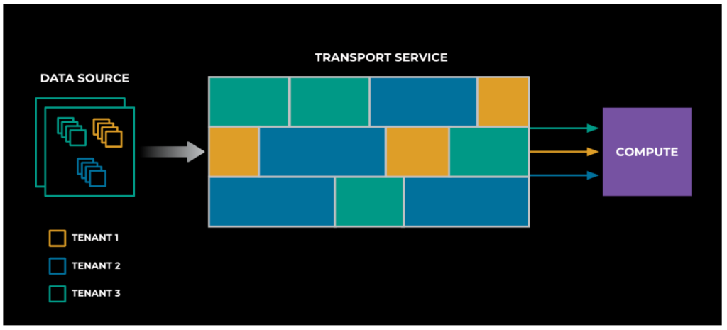
At a high level, the platform can be described as having three main components:

• Data Sources: Where the data is originally stored.
• Transport Service (the focus of this post): For each use case, it continuously reads data from the source, calls a corresponding function in the compute runtime via Thrift RPC, and tracks the progress of processed items (i.e., it does checkpointing).
• Compute Runtimes: Various environments for function execution, available as thrift endpoints.

Moving data around is a common problem in modern backend systems, and responsibility/implementation of Transport Service might look trivial. However, building it for a self-managed system with thousands of tenants can be tricky. Some of the challenges we’ll explore here may also be relevant to other multi-tenant platforms.

The consequences of multi-tenancy

The existence of thousands of tenants on Async Tier means we’ll have highly variable workloads on different dimensions with concurrent, massive unpredictability—so a lot of things can go wrong. This variance can be attributed to:

• Compute behaviour: Function running time can vary from milliseconds to minutes.
• Shapes and volumes of data: Payload size can vary from a couple of bytes to up to 1MB.
• Latency Requirements: Some of the workloads need to be executed near-real time, while others can tolerate multiple hours of delay.
• Highly irregular and spiky input traffic: Multiple use cases can go from zero to millions of executions per second throughout the day.

In the midst of heterogeneous behaviour from different tenants, the transport layer gracefully provides its services, ensuring all functions are able to reliably execute and noisy neighbours are kept under control through employing isolation and self-healing techniques. As with any highly available self-service platform, this shouldn’t require manual interventions from either the customers or the service operators. Further below, we’ll explore some of the strategies we employed to make this happen.

Multi-tenancy gone wrong

At any given point, Transport Service is moving workloads for several tenants, all of which share the same resources. In an ideal scenario, the system is able to serve all tenants gracefully.

In a highly multi-tenant and variant system, however, heterogeneity of tenants is the norm. Unguarded, some of the more demanding tenants would take over shared resources and inhibit other tenants’ progress (i.e., the Noisy Neighbour problem).

Without a proper scheme for resource sharing, adding more capacity by horizontally scaling doesn’t help, as the same pattern can (and will!) repeat at a larger scale. In the next sections we’ll review some strategies for ensuring that the system behaves gracefully under high-variability and heterogenous circumstances while ensuring tenants have the required isolation to achieve the desired throughput.

Transport Service as logical units: sharding

To understand the core of the multi-tenancy work, think of the transport layer as logical units, or shards, each responsible for continuously transporting a subset of the workloads per tenant. The union of all those units comprises our entire transport layer.

We are then faced with three questions:

• How do we isolate units to ensure each tenant operates reliably despite the behaviour of others? 
• How do we decide the number of units per tenant?
• How do we avoid fragmentation and maintain optimal resource utilisation of the fleet?

Hard Isolation

In systems with hard isolation, units from different tenants don’t share the same process. They could be deployed on different containers or physical hosts.

Since shards are hard isolated, this method is easy to set up and maintain. However, it is less efficient due to potential resource fragmentation: Not all tenants will be able to utilise a whole container, and remaining resources will be wasted. Another downside is that depending on the underlying technology, provisioning new containers (or even physical hosts) could be relatively slow and unacceptable for fast-moving, low-latency use cases.

Soft Isolation

An alternative approach is to put shards that serve different tenants in the same container and implement logical isolation on the application layer itself. 

In this setup, fragmentation is eliminated, leading to a higher resource utilisation. Shards can also be added or removed from a process quicker, leading to a faster scaling story. However, this approach comes with additional complexity in the application layer to make sure that resource contracts are well respected for each shard and the noisy neighbour problem is under control. Achieving those goals without a solid foundational framework for sharding is a non-trivial task.

Implementing softly isolated sharding with ShardManager

ShardManager (aka SM) is a generic sharding framework at Meta that assists in application shard placement, load balancing, fault tolerance, maintenance, and scaling following a policy spec written by application owners.

At a high level, SM integration works in the following way:

• Transport Service automation generates a spec file that contains a list of all tenants of the system.
  
• Each tenant is represented by a shard that can have multiple replicas. The number of replicas is dynamic, and the SM scaler component decides that number in cooperation with Transport Service based on exported load metrics and a scaling policy.
  
• Transport Service’s containers are homogeneous; they are not aware of particular tenants that they could serve. Instead, they implement “Add/Drop Shard” thrift endpoints, which allow SM to dynamically distribute shards across the fleet and move them around freely to achieve optimal utilisation and not compromise on isolation between tenants.
  

ShardManager is a powerful framework, offering multiple capabilities for various multi-tenancy scenarios. You can find out more in this separate detailed post.

Key takeaways from sharding

• Baking the concept of multi-tenancy into the system earlier is beneficial for both future scaling and current day-to-day operations such as resource provisioning, capacity management, and even monitoring/alerting.
  
• Hard isolation via separate containers and automation to provision them per tenant offers a reasonable compromise between efficiency, engineering complexity, and operational costs.
  
• Additional investments in soft isolation via application layer frameworks (e.g., ShardManager at Meta) result in  significant returns in cases involving large-scale or low-latency requirements.

Resource provisioning

By breaking down the shareable resources in Transport Service into shards, we achieve isolation among the tenants. However, we still need to dynamically provision and scale these shards individually for each tenant. 

As mentioned above, parameters such as resource utilisation, time-to-complete computation, and the rate at which workloads are generated at the data source keep changing over time. This leads to the need for a dynamic provisioning system that will enforce fairness of resource distribution without compromising SLAs for each individual tenant. 

Auto-scaling Factors

Scaling a system that serves asynchronous queue-backed traffic is different compared with scaling one that serves real-time user requests. In the case of Async Tier, one feature is the ability to build backlog in the queue and consume it during off-peak hours, when underlying compute cost is lower. Our previous blog post contains a detailed explanation of this and other usage patterns of the platform. In the above scenario, although the demand is high (queue has large backlog), compute resources are limited and scaling the Transport Service further won’t improve the throughput of the system.

To summarize, for scaling queue-backed systems it’s important to look at various factors:

• Size of the upstream queue or the amount of data to read from external data sources.
• Resource utilisation of Transport Service itself.
• Downstream backpressure: acceptance of the workloads by the compute layer, meaning this particular use case has enough allocated compute resources (such as quota, concurrency, etc). 

How much buffer to keep?

Accurately estimating the amount of resources needed for highly variadic and spiky tenants is a challenging problem to solve. Not provisioning enough resources can lead to overload and can compromise the SLAs, while provisioning too many resources will lead to low utilization and potential isolation issues.

• To solve the above problem, one can combine two approaches: For non-latency-critical workloads, reactively auto-scale and rely on overload signals with minimal buffers. Even if it takes some time for a specific shard to scale up, the system would still meet its SLAs.
  
• For latency-critical, spiky workloads, there is no option but to keep a larger buffer and make it clear to customers that lower-latency SLAs come at the higher cost of an extra resource buffer.

Key takeaways from resource provisioning

• Efficient and reliable auto-scaling for queue-backed asynchronous workloads has to consider upstream and downstream factors along with utilisation of the service itself.
  
• Auto-scaling is always a tradeoff between SLA misses and efficiency. One way to make it less painful is to use soft isolation between shards and incorporate latency/spikiness in the cost model.

Downstream protection

Transport Service is also responsible for ensuring the health of the compute layer downstream while preventing workload data loss. This becomes challenging to maintain in events involving downstream degradation, as described below. 

The compute layer can degrade due to numerous factors. Some of the most common are:

• a particular use case running out of allocated resources (such as quota, hitting concurrency limits, etc.)
• a bug in the function code on compute side, causing widespread failures
• temporary global outages in one of Meta’s internal services. Given that Async Tier is one of the highest sources of traffic to services such as TAO (Meta’s social graph data store), it should swiftly react to such degradations, allowing downstream a chance to recover while serving realtime user traffic.
  

In all of these cases, Transport Service starts experiencing throttling of the RPCs to the downstream and needs to reduce the ingestion rate by slowing down. It also needs to continue retrying already-rejected RPCs to prevent data loss, probe for recovery signals, and (once it recovers) eventually increase the flow to utilize the downstream to full capacity. This behaviour is usually called flow control. In the next section we will explore various approaches to implementing reliable and efficient flow-control mechanisms.

Backoff and retries

Retrying failed RPCs in place can lead to a retry storm and overload the downstream even further, which can exacerbate the degradation and significantly slow down the recovery. Adding a fixed backoff interval has similar downsides—it will cause retry spikes, as retries will likely share the common backoff interval coefficient from the point of time when degradation occurs.

While this does allow the downstream some intermittent recovery time, the load spikes can still impede its restoration. Spreading the retries with some “jitter” can alleviate these spikes—Figure 11 illustrates the jitter as random intervals added to the fixed backoff to spread the retry load more evenly.

Adaptive flow-control

Degradation incidents are non-deterministic, however, so it is hard to predict effective parameters for these retry strategies. Moreover, since our use case involves an asynchronous computation platform, we had the flexibility of a relaxed SLA to execute the tenants’ entire workloads. These nuances pave the way for a flow-control strategy that can keep increasing the traffic to target optimal utilisation of downstream resources. Eventually that increased flow will cross the threshold that triggers throttling;  then reacts quickly to decrease the flow and facilitate recovery. We implemented this with a budget-based, flow-control strategy.

Here’s a simplified explanation of this strategy: Each RPC consumes one token from the pool. If tokens are not available, RPCs will be queued up. In reality, the token assignment to RPCs should not be 1:1 but weighted according to the amount of resources they might consume on the compute, but for this explanation let’s assume it’s 1:1. After successful completion of execution, the token is returned to the pool. Over time, as we continually experience successful completions of the RPC, we gradually increase the pool size, thereby increasing the flow to downstream. However, as soon as we experience throttling or signals of overload, we restrict the flow by aggressively decreasing the number of tokens in the pool. The aggressive decrease is important, as degradation incidents accelerate fast. In our platform, we implement this using AIMD (Additive Increase Multiplicative Decrease). Over time this approach forms a cycle of gradual flow increase, throttling, rapid decrease, and recovery—and thus dynamically controls the flow from Transport Service to downstream.

Key takeaways from downstream protection

• Backing off with jitter can prevent major operational issues caused by downstream outages, but will be harder to maintain/configure for diverse multi-tenant systems with huge variance in workload characteristics.
  
• Adaptive (budget-based) flow control is harder to implement, but it can achieve optimal efficiency and accuracy compared to straightforward alternatives.

Conclusion

The technical challenges described in this post are generally relevant for any multi-tenant backend system that transfers data among multiple sources and destinations. But there is one important aspect to consider before applying the solutions presented here. When working on scaling and optimizing things, there’s a natural tendency to begin by optimizing as much as possible. As a first step, however, it’s always a good idea to speak with the customers and align with their expectations and business needs before investing in significant changes like the ones we have described. This will help your engineering team focus on business-critical aspects of the system first, and guide you in choosing the right trade-offs in terms of complexity, capacity usage, and operational modeling within the agreed SLAs.