


Introduction
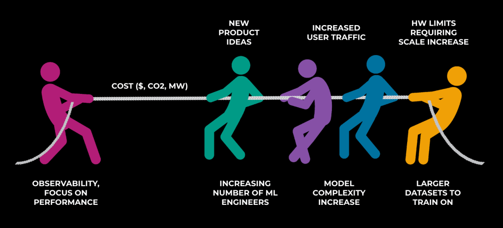
The latest advancements in AI and the promising results delivered by many of our flagship models justify making considerable investments in scaling up our AI-focused infrastructure. As illustrated in the following diagram, many factors drive up the cost of that infrastructure, including new products, increased model complexity, larger datasets, and simply hiring more machine learning (ML) engineers to run experiments.
One of the relatively few levers against exponentially growing costs is our focus on efficiency. In the scope of this blog, efficiency refers to the combined efforts focusing on the performance of the software stacks and the underlying hardware infrastructure. When models may take hundreds of thousands of dollars to train a single combination of hyperparameters, investing in accelerating those jobs may yield significant cost savings. The cost metric can be in dollar amounts, megawatt footprints, and CO2 emissions.
The key to enabling all the efficiency work is observability. We consider observability the conglomerate of technologies, tools, datasets, and dashboards that enable us first to evaluate the level of performance achieved by our infrastructure at different granularity levels and then to guide us where to invest.
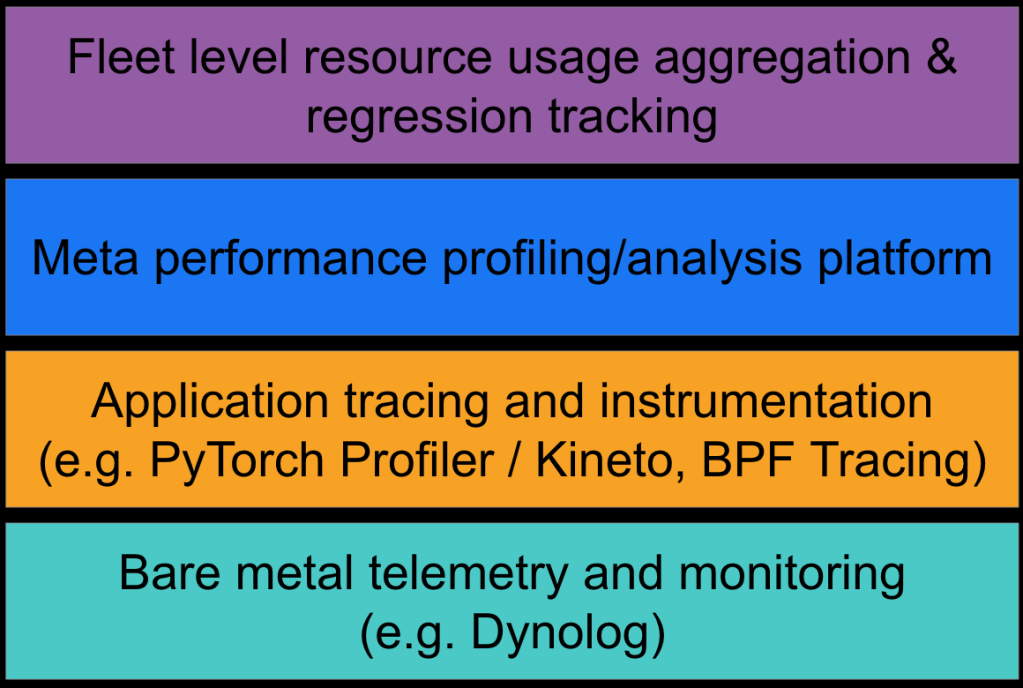
In this blog post we will describe the fundamental layers of Meta’s AI observability infrastructure along with some of the challenges and capabilities of our tools. We believe our solution covers a wide spectrum of capabilities that enable us to have accurate resource usage attribution at a high level, and also provide detailed performance introspection at the job level.
- The support layer of our observability is the bare-metal telemetry and monitoring. This layer enables us to collect the bare-metal metrics that we can use to estimate the level of performance achieved by an application, and furthermore to build all the datasets where we aggregate resource utilization.
- Next we have a set of tools that we can use for advanced performance introspection. Tools such as PyTorch Profiler, Kineto, and Strobelight/BPF are typically used to trace the application and identify bottlenecks or various issues (for example, memory leaks).
- The third layer moves towards scaling out performance introspection. At Meta scale we have tens of thousands of jobs that execute daily, hundreds of models, and thousands of ML engineers. By contrast, the number of AI performance experts is lower by orders of magnitude. Therefore, with tools such as Meta Performance Profiling/Analysis Platform, we aim to collect and aggregate profiling data from various profiling tools, as well as hardware-level utilization and job-level performance metrics. Moreover, Meta Performance Profiling/Analysis Platform automates the process of analyzing collected data and then pointing to the main performance issues. Commonly found anti-patterns can be highlighted at this layer, allowing AI performance experts to focus on more complicated use cases.
- Finally, the fourth layer aims to use the generated datasets at the entire fleet level to build dashboards/visualizations that guide optimization work and support the decision process regarding how we are building infrastructure and software tools.
Monitoring & Telemetry
Over the years, Meta capacity has grown exponentially to encompass 21 datacenters. To ensure our services run properly and efficiently, telemetry observability is an indispensable prerequisite.
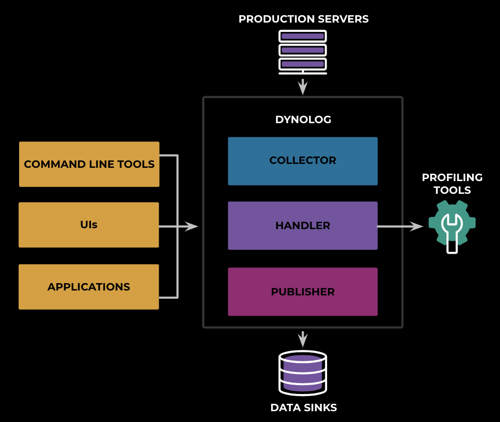
Dynolog is our distributed telemetry daemon running on all Meta’s hosts. It fulfills several important roles:
- It collects system telemetry at the host/process level.
- It collects workload metadata and conducts resource accounting to the proper workload owner.
- It functions as a server for real-time telemetry queries to support use cases such as load balancing and autoscaling.
- It serves as the moderator of the telemetry tools on the host to interact with remote on-demand user requests.
Dynolog Architecture
As a brief overview of the system, Dynolog monitors the system telemetry through the following modules: collector, publisher, and handler. The collector interacts with system/vendor APIs to collect telemetry signals periodically, and it aggregates the metric at the publisher to send to multiple data sinks (real-time ODS, Scuba, and Hive). The handler listens to RPC communications, retrieves the desired data from the collector for application real-time usage, or forwards the request to other profiling tools such as trace collectors.

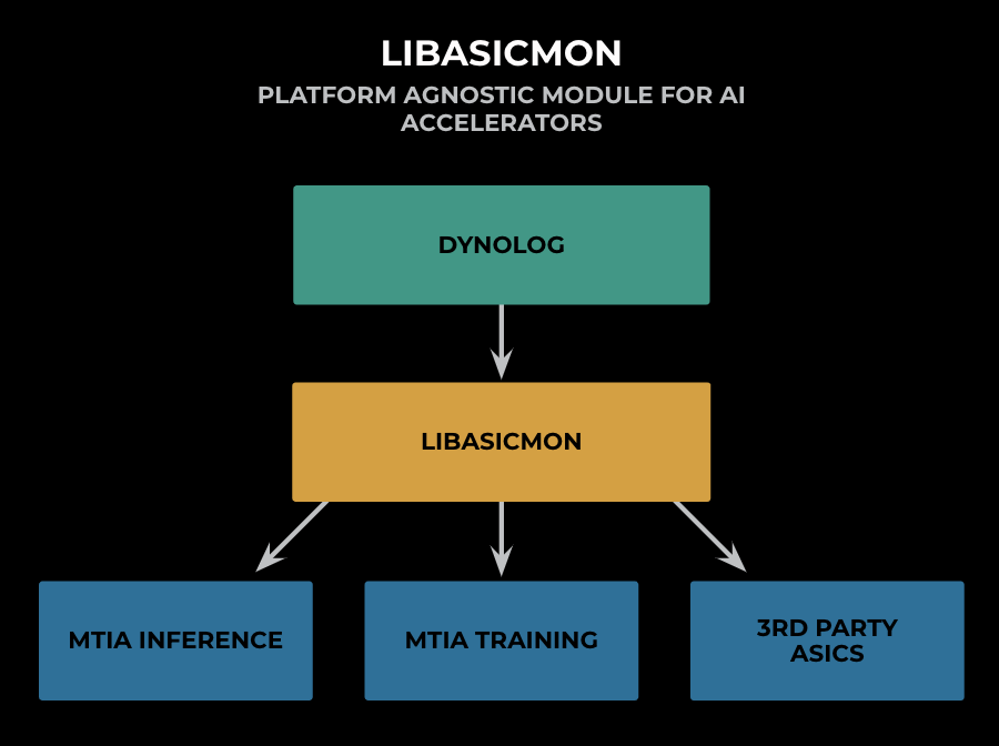
One major challenge of AI observability comes from the heterogeneity of the fleet. As the computational demand increases with the complexity of AI workloads, the heterogeneity of the fleet increases with the deployment of various application-specific integrated circuits (ASICs), including the Meta Training and Inference Accelerator (MTIA), third-party vendor ASICs such as GPU, inference accelerators, and video encoder/transcoders. To address the challenge, the Dynolog collector module generalizes the metric collection and configuration through LibAsicMon, a platform agnostic observability system for AI accelerators. This provides a scalable way of surfacing significant efficiency metrics for the AI fleet, and it enables customization for individual ASICs without exposing the complexity of interacting with individual vendor/firmware APIs.
Dynolog also has open-source support with system telemetry and DCGM GPU monitoring features, and it has been used in non-Meta production environments such as the FAIR research cluster and lab environments for new hardware testing. Please see https://github.com/facebookincubator/dynolog for more details.
Topline Efficiency Metrics
The telemetry system provides observability of multiple efficiency signals ranging from device health and power to individual compute-processor utilization. These bare metal utilization and device metrics provide a strong indication of efficiency when used in a good combination. The question now becomes: What metrics are the best representations of fleet efficiency, and how to leverage them for efficiency work?
| Metrics | Correlation to Model Complexity Growth | Correlation to HW generations | Correlation to efficiency work | Create bad modeling incentives | Collection technical challenge |
| FLOPs/sec | High | High | High | Yes | Average |
| Compute Unit Utilization | Medium | Medium | Non-linear | No | Low |
| Device Power | Medium | Medium | High | No | Low |
| Device Utilization | Low | Low | Medium | Yes | Low |
| rDevice hour / Byte | High | Medium | High | No | Average |
| % of Roofline | Low | Low | High | No | Difficult |
The column Create bad modeling incentives represents how adding bad model design could lead to an increase of the signal, which in turn could lead to workload owners increasing the metric through bad design practices (for example, we can add more dense layers to increase FLOPs/sec).
The chart illustrates that FLOPs/sec correlates best with the efficiency and complexity of the model and HW generations while presenting feasible implementation challenges. We use FLOPs/sec as the topline efficiency metric with Compute Utilization and Power to alleviate FLOPs/sec’s bad model incentives.
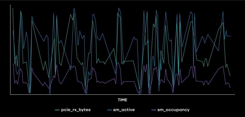
Using the Nvidia GPU as an example, we leverage DCGM to collect device power, performance signals at the GPU-device level, SM level, warp level within SMs, and derive FLOPs/sec based on a heuristic estimation. These signals give a comprehensive view of the workload performance through three layers of granularity, and they are continuously collected at fleet level with very low overhead, providing a well-rounded foundational picture of the fleet performance.
The chart above also displays two metrics that are not well known. One is rDevice hour/Byte. This is a derived metric that tries to measure the amount of compute time per byte of input; with it we are trying to determine a normalized cost metric that correlates well with efficiency efforts but that does not create bad modeling incentives. For example, FLOPs/sec may tempt ML engineers to increase the linear layers` count or sizes in order to show high FLOPs/sec usage, but this may not be the best path to unlock model quality gains.
The best metric for evaluating a given workflow’s performance is the percentage of its roofline performance. This is a more advanced metric and requires traversing the device timeline, writing analytical roofline models for all device kernels, assuming a large reduction in idle time between kernels, and then comparing the roofline duration with the actual execution time.
FLOPs/sec Estimation
Unlike CPUs where FLOPs are well supported by hardware counters, ASICs present more challenges in collecting and estimating FLOPs. The hardware counters don’t provide the same level of information, and the measurement and the techniques for collecting them raise additional challenges (including high overhead, kernel replays, and workflow failures). As an example, Nvidia GPU doesn’t provide hardware counters on floating-point operations, which makes measuring FLOPs on GPU hardware cumbersome. To address this, we identified the following two approaches to estimate FLOPs.
DCGM
Nvidia’s Datacenter GPU Manager (DCGM) provides continuous measurement of individual ALU utilization, so we estimate the FLOPs/sec by multiplying the peak throughput of each utilization unit and then calculating their total sum.

To make the problem more challenging, the tensor core unit supports multiple precision formats with different peak throughput, and there is no accurate way of determining which precision format is used for an application. To resolve this problem, we applied the following heuristic: FP16 activity / FP32 activity > threshold. If the FP16 pipeline shows increased activity, there is a higher chance that the tensor core unit is executing FP16 instructions.
CUPTI
The CUDA Profiling Tools Interface (CUPTI) provides APIs to collect executed FLOPs for a given workload iteration, using a combination of hardware counter and binary instrumentation. It enables accurate measurement of FLOPs, but enabling it continuously or at fleet level results in high overhead.
Accuracy
We use CUPTI measurement as a benchmark reference for DCGM-estimated FLOPs and see results less than 10 percent higher than those from DCGM. The inaccuracy comes from three main sources:
- The FP16 and FP32 pipeline-utilization metric increases when executing a subset of integer instructions.
- The pipeline-utilization metrics only measure the number of busy cycles, but the floating-point instructions have similar latencies between ADD, MUL, and FMA instructions. We currently assume we are executing FMA instructions.
- Tensor core instructions have multiple precisions and we rely on heuristics to assume a specific format.
Based on the heuristic estimation from DCGM, we are able to collect FLOPs/sec at the fleet level with negligible overhead and reasonable accuracy.
Automated Performance Introspection & Debugging
End-to-End Profiling
System performance is the result of interaction across different layers of the stack. At Meta we use various tools to understand the performance and interactions across these layers.
For example, a workflow might make a call over the network to get some data, do some processing on the host (CPU), and call a Kernel on the device (GPU). To get a holistic view of system performance, we want to understand the time spent in the network call, CPU processing, queuing the call on the device, and the actual execution start and end times on the device. Using this data we can identify bottlenecks, understand inefficiencies, and identify opportunities for improvement.
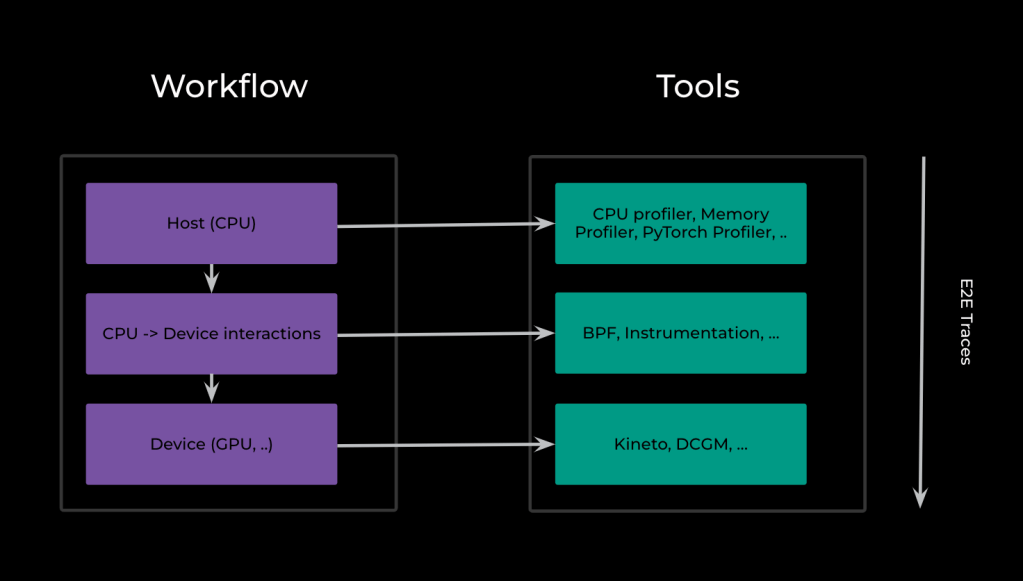
Three main sources of profiling information used at Meta are Kineto, PyTorch profiler, and Strobelight.
Kineto
Kineto is a CPU+GPU profiling library that provides access to timeline traces and hardware performance counters. It is built on top of Nvidia’s CUPTI. We rely on Kineto for information on kernel executions, memory operations, and utilization metrics for various hardware units.
Kineto is open sourced and integrated into PyTorch Profiler.
PyTorch Profiler
PyTorch Profiler is another tool we rely on for profiling our workload performance. PyTorch Profiler allows the collection of performance metrics during training and inference. It is used to identify the time and memory costs of various PyTorch operations. Depending on how you run it, PyTorch Profiler can collect all these metrics, some of them, or none at all.
Strobelight
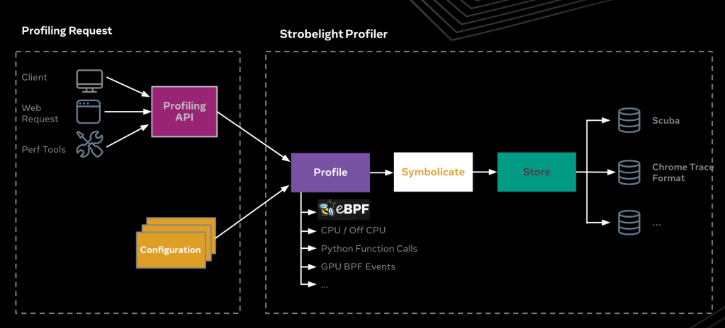
Strobelight is a daemon that runs on all of Meta’s fleet hosts and acts as both a profiler and a profiler orchestration tool. Profiling can be triggered by certain events (such as an OOM event), runs on a pre-configured schedule or on-demand.
Strobelight is composed of multiple subprofilers. Through these subprofilers it
has the ability to collect various performance profiles such as CPU stack traces, Memory Snapshots, and Python stack traces from any host in the fleet.
Strobelight relies on eBPF (or simply BPF) for many of its sub-profilers. And we have recently added a BPF-based CPU -> GPU profiler to Strobelight’s profiler suite.
Using BPF for performance profiling AI/ML workloads
In a nutshell, BPF is Linux kernel technology that can run sandboxed programs in a privileged context such as the operating system kernel.
Why BPF?
Using BPF for profiling and observability has many benefits. To name a few:
- Security: BPF Verifier ensures that the BPF programs are safe to run, will not cause crashes or harm the system, and will always continue to completion.
- Programmability: BPF provides a safe, in-kernel, highly programmable environment.
- Low overhead: The overhead for attaching probes to user-space functions (uprobes) is minimal, and when the uprobes are not attached there is no impact to the application performance.
- No need for instrumentation: BPF can attach to and profile user-space and kernel events without instrumentation. While instrumentation can be added to provide additional context or make the BPF program resilient to code changes, most BPF programs work out of the box.
Gpusnoop
Gpusnoop is a BPF-based profiler suite that Strobelight supports. It can hook into a variety of interesting GPU events such as cuda kernel launches, cuda sync events, and cuda memory events. It also supports profiling PyTorch memory events.
Use Case: Profiling cuda memory allocations using BPF
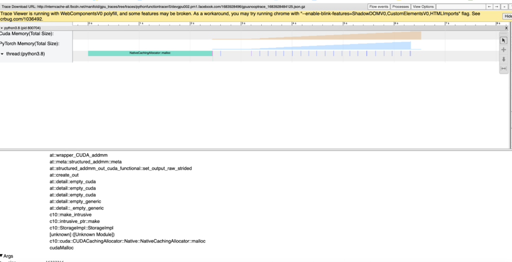
By attaching to CUDA memory allocations and CUDA memory-freeing events using uprobes, gpusnoop can be used to build a timeline of memory allocations and detect the stacks of unfreed or leaked memory.
The (simplified) code below will attach to cudaMalloc and cudaFree events and record all freed and unfreed memory allocations, along with their sizes and stacks.
User Space:
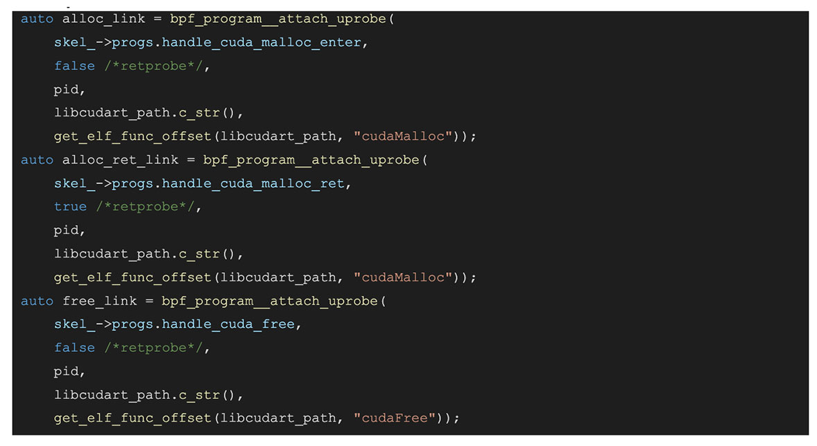
BPF Space:
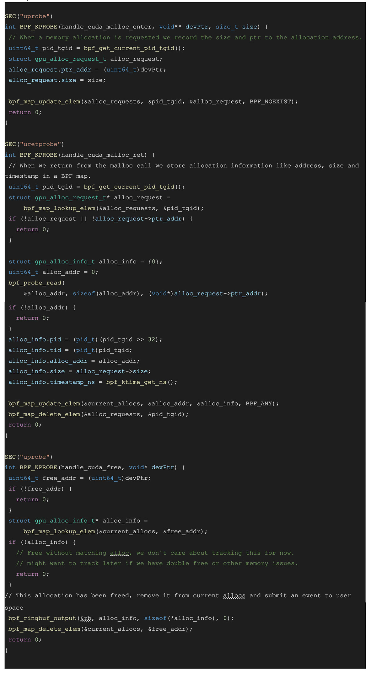
The code above attaches to cudaMalloc enter and tracks the requested allocation size, then attaches to the cudaMalloc return and grabs the allocation address after it’s been set. It uses this data to keep track of the outstanding allocations and their sizes. We can then use this data to track the outstanding allocations and their sizes and stacks at any point of time. We can also visualize this data and detect things like the memory leak in this example or use it to narrow down the stacks using the most memory.
Since PyTorch has its own memory manager, the code above can be expanded to attach to PyTorch memory allocation events by simply attaching to different functions in the user space.
Automated Trace Collection
Most of our jobs will run on more than one host and process at a time, and will require data from more than one profiler. Our Automated Trace Collection systems handle trace collection from multiple profilers across multiple hosts.
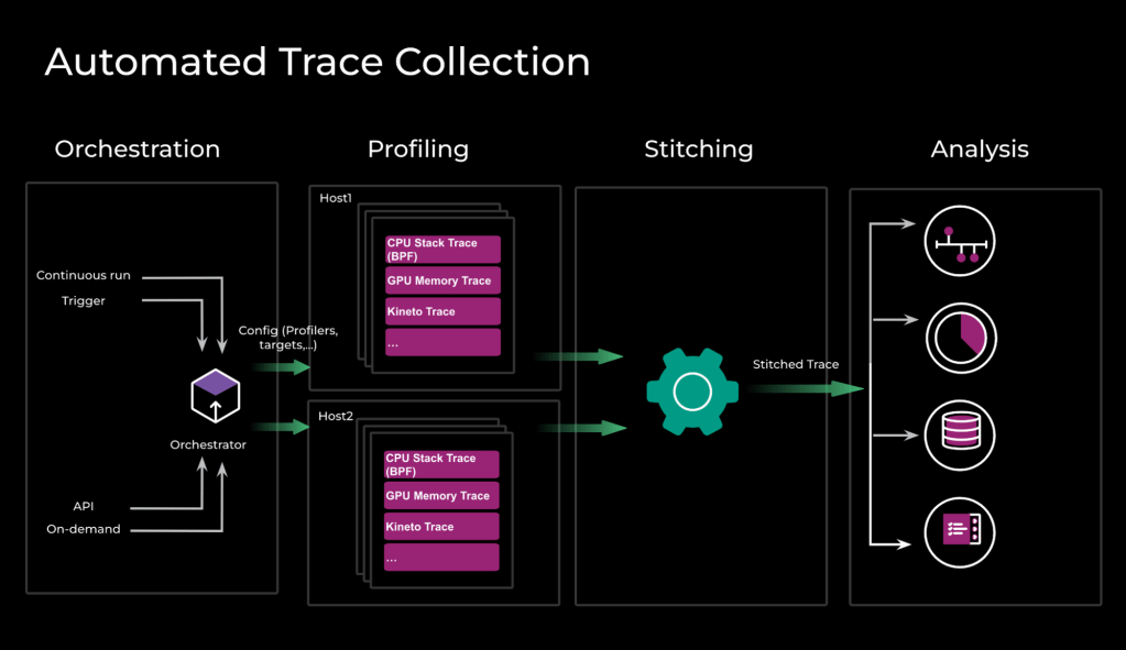
Automated Trace Collection involves four different phases:
- Orchestration: We determine which profilers and hosts we will be running during a profiling run; each run will have a trigger, a configuration, and one or more targets.
- Triggers can be an API call, an interesting event like a performance counter hitting a certain threshold, or a continuous-run configuration that runs at a certain cadence.
- This step also ensures that all profiler starts are synchronized across different hosts.
- Profiling: Once the targets (for example, hosts or processes) are determined, a run request is issued to each host with the run configuration, and the orchestrator will wait for the runs to finish.
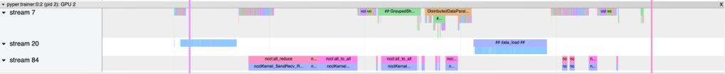
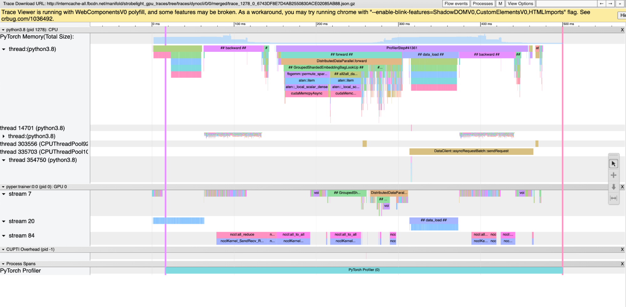
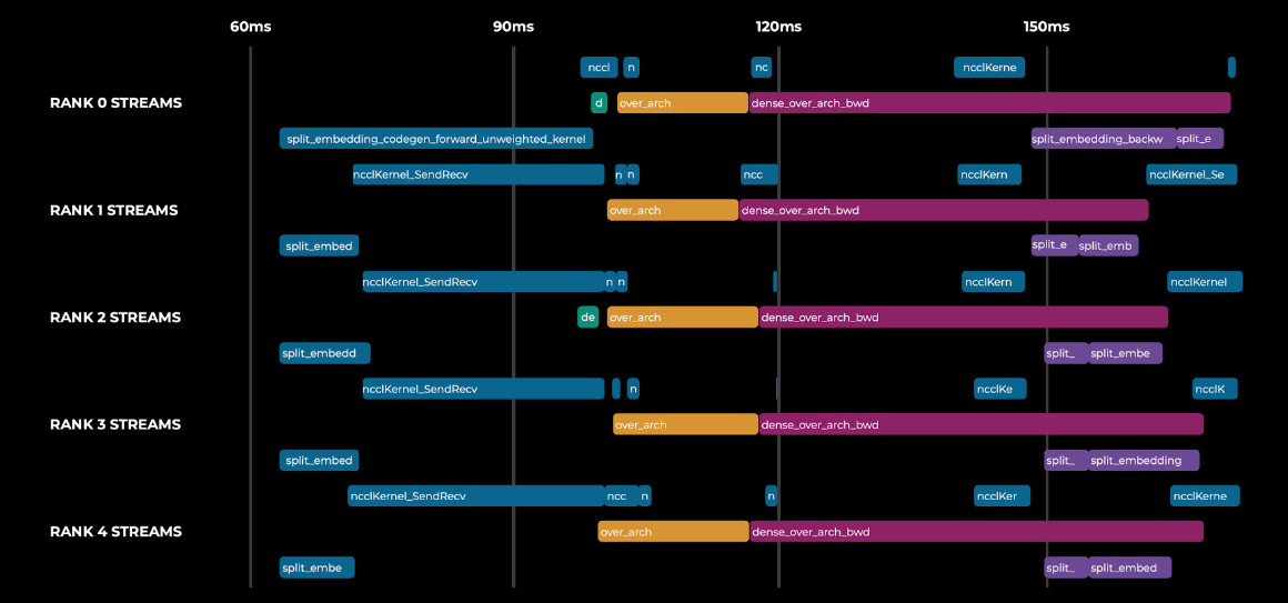
- Stitching: Once we have received results from all runs, the orchestration “stitches” the traces. This means combining data from multiple sources into a single holistic view. In this figure we can see the memory allocations, python function stacks, gpu events, and PyTorch events in a single timeline.
- Analysis: This data is then used for building timelines, performing auto-analysis, or identifying improvement opportunities.
Meta Performance Profiling/Analysis Platform
Overview
Meta Performance Profiling/Analysis Platform is an automated, one-stop shop, self-service platform for performance profiling, analysis, insights, and action for AI workloads at Meta. It started with the idea of profiling-as-a-service and then evolved to become a platform focused on usability. It is seamlessly integrated into Meta AI development and production environments.
Example Features
Auto-Profiling and On-Demand Profiling
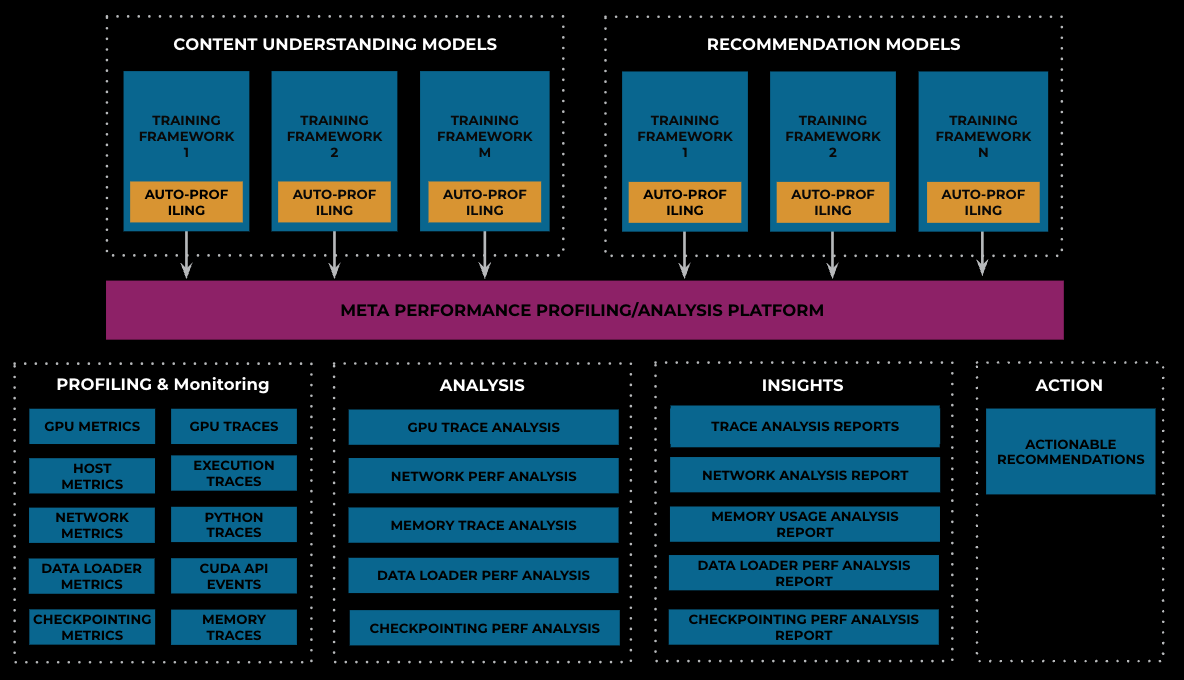
Meta Performance Profiling/Analysis Platform automatically collects and aggregates profiling data from various profiling tools, along with hardware-level utilization and job-level performance data. Adding the auto-profiling thrift call into the training loop for a framework, Meta Performance Profiling/Analysis Platform automatically profiles every job created by the framework, and then creates a profiling report. Through such a seamless integration with various training frameworks of recommendation models and content-understanding models, Meta Performance Profiling/Analysis Platform profiles fleet-wide training workloads. In order to debug performance variations during the training process and support training frameworks without the auto-profiling support, Meta Performance Profiling/Analysis Platform also supports on-demand profiling support, which can be triggered manually via the Performance Profiling User Portal.
- Workflow
In the Auto-Profiling case, the performance profiling service receives a profiling request thrift call from a framework. It downloads the traces of the target job from the Object Store according to the trace-location information stored in a predefined table. In the meantime, it reads host metrics, GPU metrics, and GPU host network metrics from data sources stored in relevant time-series telemetry tables. Once all the profiling data is gathered, Meta Performance Profiling/Analysis Platform performs a series of analyses, generates a profiling report, and writes outputs to performance DB tables. Finally, Meta Performance Profiling/Analysis Platform delivers an overall profiling report with detailed and insightful analysis to the user.
Auto-Analysis & Insights
Meta Performance Profiling/Analysis Platform automatically analyzes collected profiling data and generates analysis reports. There are two major categories of profiling data: traces and metrics. Meta Performance Profiling/Analysis Platform runs trace analysis tools such as Holistic Trace Analysis/Automated Trace Comprehension to analyze GPU traces, execution traces, python traces, CUDA API traces, and memory traces to identify performance bottlenecks and issues. On the other hand, Meta Performance Profiling/Analysis Platform also scans the collected GPU metrics, host metrics, network metrics, and data loader metrics to evaluate performance and resource utilization, as well as detect abnormal outliers.
- Insights
For a profiled job, Meta Performance Profiling/Analysis Platform creates analysis reports and presents important insights to the job owner to ensure that the analysis results and found issues are easy to understand. Through trace analysis, Meta Performance Profiling/Analysis Platform is able to reveal hidden performance issues, including load imbalance among workers due to an imbalanced sharding plan, GPU idleness due to data starvation, training being CPU-bound due to synchronization points, and so on. All the insights and findings are used to provide actionable recommendations to users to fix performance issues and improve training performance and efficiency.
Trace-Based Fleet Level Workflow Characterization
Our automated trace collection systems collect tens of thousands of GPU traces daily that contain valuable information about the specific workflows we execute in the fleet. By doing data mining on the traces, we can extract valuable data points that indicate the major bottlenecks of our workflows, how we can adjust our hardware infrastructure to provide better ROI, and which software investments can maximize the infrastructure utilization efficiency.
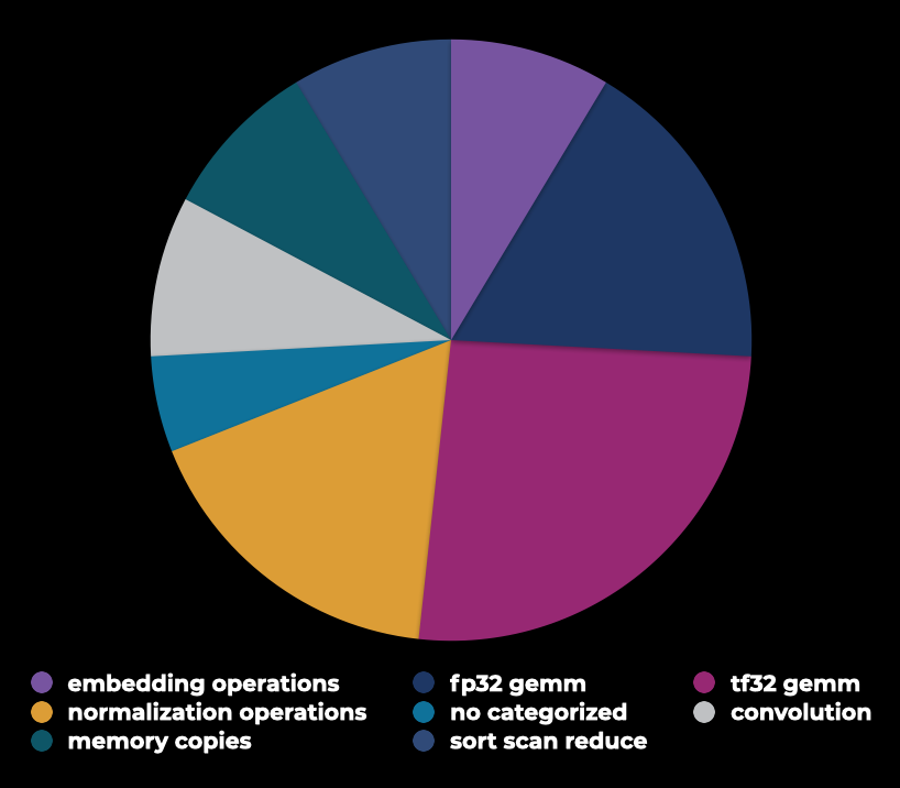
One such data point is a breakdown of GPU time by compute type. We can see how compute cycles are distributed among operations that are bottlenecked by the memory bandwidth of floating-point operations’ throughput. In addition, we see the GPU code that is being called most frequently in our fleet. This information will be very useful in trying to build efficient infrastructure over the next few years.
Another valuable datapoint tracks the average duration of GPU kernels across an extended period of time, allowing us to observe any regressions. For example, in the image below, we can observe that embedding table lookup kernels have suddenly increased their duration by orders of magnitude. We can then deep dive into the jobs that express this behavior and fix any related issues. Given that each of the kernel samples have sufficient metadata for us to trace back to the job that shows the regression, we can use Meta Performance Profiling/Analysis Platform to gain a complete view of the performance profile.
The same dataset can be used to guide device-code optimizations in frameworks such as PyTorch. For example, we can rank kernels by their device-cycles footprint throughout the fleet. We can then investigate each important kernel code and look for potential opportunities. One of the next developments is to collect input sizes for the PyTorch kernels. This information will highlight whether there is potential for writing specialized implementations for widely used problem sizes, for which we can simplify the code paths and have stricter control over resources such as local memory, register usage, and more.
Fleet-Level Resource Attribution
One challenge of guiding efficiency work is attributing resource usage per various entities. These can have different granularities, including job, user, model, product, division, application type, or base framework. This attribution allows us to decide where to invest effort in optimization. Using the basic telemetry described in the previous sections, we have built a suite of dashboards that eventually illustrate a view like in the figure below:
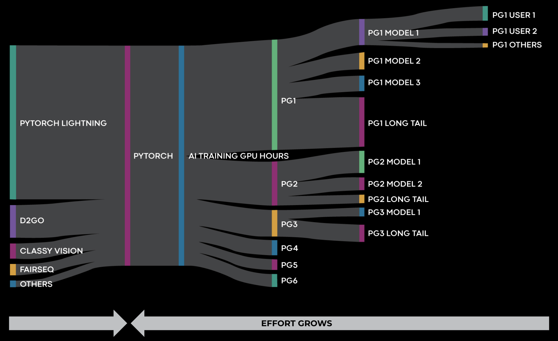
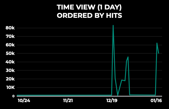
The diagram reads as follows: We run applications for a number of GPU hours during a selected interval. These GPU hours are split among product groups, models, users, and eventually jobs. If we detect, for example, a specific model that has a large number of GPU hours, we can also observe a timeline of its usage for an extended period. GPU hours are closely tied to infrastructure operating costs, so using this attribution we can invest optimization efforts in the most resource-consuming areas.
Similarly, we can do this breakdown per framework type. We serve multiple use cases within Meta, and software stacks that have particularities specific to those use cases would require specific optimizations.
An important thing to note is that while framework improvements might be preferable, since they have the potential to accelerate all jobs, usually framework-level wins are marginal after a certain level of maturity. In contrast, models tend to constantly expose large optimization potential due to their constant shape shifting. In some cases, model optimization work will have higher ROI than framework-level wins.
Acknowledgments
Building AI Observability at Meta scale needed significant teamwork and management support. Hence, we would like to thank all contributors to the project. A special thank-you to Wei Sun, Feng Tian, Menglu Yu, Zain Huda, Michael Acar, Sreen Tallam, Adwait Sathye, Jade Nie, Suyash Sinha, Xizhou Feng, Yuzhen Huang, Yifan Liu, Yusuo Hu, Huaqing Xiong, Shuai Yang, Max Leung, Jay Chae, Aaron Shi, Anupam Bhatnagar, Taylor Robie, Seonglyong Gong, Adnan Aziz, Xiaodong Wang, Brian Coutinho, Jakob Johnson, William Sumendap, Parth Malani, David Carrillo Cisneros, Patrick Lu, Louis Feng, Sung-Han Lin, Ning Sun, Yufei Zhu, Rishi Sinha, Srinivas Sridharan, Shengbao Zheng, James Zeng, Adi Gangidi, Riham Selim, Jonathan Wiepert, Ayichew Hailu, Alex Abramov, Miao Zhang, Amol Desai, Sahar Akram, Andrii Nakryiko

