





A data center network begins life as a logical diagram: this many spine switches, connected to this many fabric switches, in this fabric topology. Building it means answering two much harder questions. Which of the thousands of rack positions should each device occupy, given the power, space, and failure domain of each? And which of the millions of fiber strands should connect them, through which panels, cassettes, trunks, and breakouts? Traditionally both answers came from engineers working by hand, from judgment never written down.
At Meta we built a Design Automation Pipeline to automate that work. We broke down the end-to-end design process into its individual components. One component of this pipeline, Planogram, places every network device and AI rack onto the floor plan subject to dimensional, power, and failure-domain constraints; another component of the pipeline, fiber design automation, turns the placed plan into a fully specified fiber plant, down to every cable, connector, port, and strand, plus a build-ready bill of materials. Together they compress physical network design from months to days, and re-validation from days to minutes.
Why physical design became the bottleneck
For most of the past decade this was not the hard part: Meta built to a handful of standardized designs, and when the floor plan repeats, placement and fiber are close to templates. Three shifts broke that.
- Volume and speed. McKinsey estimates 18 GW of new capacity will be needed industry-wide in 2026 alone, with hyperscalers targeting 30–50% shorter build cycles.
- Heterogeneity. Space and power now bind hardest, so capacity is sourced wherever it exists, and every non-standard floor plan is a fresh problem.
- Optionality. Floor positions are eligible to serve either server or network hardware.
- Design proliferation. AI workloads do not share one topology, and the accelerator roadmap turns over every 12–24 months, so designs are re-pivoted late and often.
It lands on a process that runs early: physical design starts 12–18 months before production traffic, because its bill of materials drives long-lead fiber ordering. Done by hand, the arithmetic stops working, and on both halves of the problem at once (Table 1). None of those challenges occur once—they recur every time a rule, a topology, or a floor plan moves, and Design Automation Pipeline today carries 100+ concurrent design variants.
| Process step | Manual | Automated |
|---|---|---|
| Initial device and fiber allocation | months | days |
| Re-allocate after a requirement change | weeks | days |
| Validation (every change) | days | minutes |
Table 1. Physical design cycle time, manual versus automated end to end with Design Automation.
Speed was never the whole problem. Manual design produced designer-to-designer variance and surfaced infeasibilities. These problems, such as an unpowerable rack row or a failing loss budget, appeared only near deployment, when they were most burdensome.
The end-to-end design pipeline
Figure 1 shows the workflow of the Design Automation Pipeline: all network equipment, from rack switches to backbone routers, plus the AI racks.
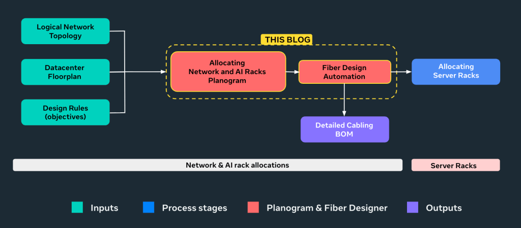
Figure 1. The end-to-end physical design pipeline. Planogram and the fiber designer are covered in this post.
Planogram consumes the logical network topology, the Datacenter floorplan, and a set of design rules, and assigns every entity a row and rack position. The fiber designer turns that placed plan into the fiber plant and the cabling bill of materials (BOM) that goes out for ordering.
Two properties matter more than the diagram suggests. Everything downstream is generated rather than transcribed, so ordering artifacts cannot drift from the design. And because Planogram runs in minutes, engineers re-run it against a perturbed stencil to see whether a small physical change unlocks a better design.
Inside Planogram: the placement optimization model
Planogram assigns every logical entity, including switches at every layer, AI accelerator racks, accessory racks to a row and rack position. Entities sharing a role are interchangeable for placement; an electrical-failure domain (EFD) is a group of racks sharing a power feed. Examples below use the standard fabric tiers for network switch roles: FSW (fabric switch), SSW (spine switch), and XSW (exospine aggregation switch). Placements must respect fixed-infrastructure limits (i.e., available positions, per-rack power, rowlet gaps) and design-driven constraints holding circuit-connected devices a bounded or fixed distance apart.
The objectives, and why they fight each other
The interesting part is not the constraints but the objectives.
- Spreading entities: spreads entities across failure domains so no failure scenario exceeds what the domain owners accept.
- Minimize connecting rack pairs: minimizes the rack pairs connected between adjacent layers, reducing fiber resource needs.
- Ensure similarity: keeps rack roles consistent across corresponding rows in different row groups.
- Ensure rack efficiency: packs entities into the fewest racks within a row group.
Take the first two. Spread every XSW plane across all failure domains and an EFD failure degrades each SSW by 25% while disconnecting none, but every SSW must then run fiber to every XSW row. Put all planes in one row and each SSW connects to one row, optimal for fiber, but an EFD failure takes an entire SSW offline. That trade-off is the design decision, and it is why Planogram has no single objective function.
A lexicographic mixed-integer program
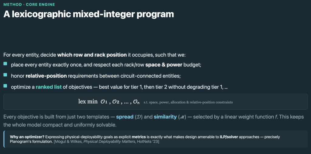
Planogram ranks rather than weights. Objectives are solved lexicographically (Figure 2): the solver finds the best value for the top-priority objective, then optimizes the second without degrading the first, and so on. Design intent becomes an ordering rather than hand-tuned weights.
The program in full
The decision variables are zqij, the number of role-q entities at row i and position j, and yrij, a binary for the rack role at (i, j). Seven constraint families do the rest (Figure 3).
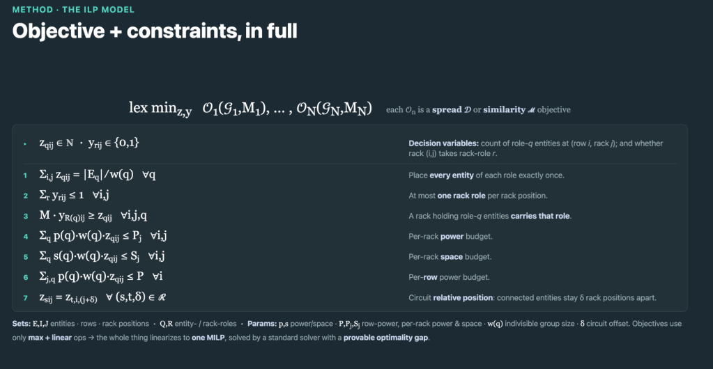
Every objective uses only max and linear operations, so the model linearizes into a single mixed-integer linear program that returns a provable optimality gap on every run. That matters: the output drives large scale orders.
Why an optimizer and not a heuristic
We prototyped evolutionary and local search early, and they plateaued below the per-tier optimum. The ILP enforces lexicographic priority by construction, reports a provable optimality gap, and expresses relative-position constraints as declarative one-liners rather than error-prone move operators.
What it contributes
A run completes in one to two minutes, and infeasible configurations are rejected in around 0.21 seconds, which makes speculative re-runs practical. The quality improvements matter more than the cycle time:
- Efficiency. Planogram optimizes a “minimize connecting row pairs” objective designers never explicitly met, cutting wasted fiber.
- Feasibility. Frontloaded space and power modeling caught an infeasibility; manual planning would have surfaced only near deployment.
- Consistency. Designer-specific conventions disappear, yielding reproducible designs across engineers and regions.
Some of this only became visible through automation: an explicit objective for every rule exposed which conventions were requirements and which were habits. We had been half-filling network racks for “future upgradability,” which analysis showed wasted space for no benefit. The hardest part was never the solver; it was eliciting objectives encoding knowledge designers had never written down.
Inside the Fiber Designer: Solving connectivity for any floorplan layout
Turning a logical topology into every cable product, panel, cassette, port, and strand historically took multiple weeks per project. Design Automation’s Fiber Design Module compresses it to minutes, consuming the LNTG, where each circuit carries an optic profile, so a 400G-FR4 needs two strands and a 400G-DR4 eight, plus the placed floor plan. Strand demand rolls up through the physical hierarchy, driving aggregation, sizing, product selection, and diversity.
The core abstraction: the channel schematic
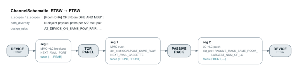
The unit of authorship is a blueprint, not a cable list. A channel schematic describes one cabling layer as an ordered chain of hops between an A-side and a Z-side device role, saying nothing about which racks are involved; the engine binds it to the floor plan at application time. The designer authors the endpoint chain, a cable-product recipe per segment, an endpoint preference, and a striping rule and the rest is derived (Figure 4).
Where does each hop land?
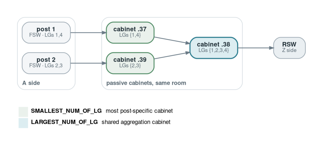
Applying a schematic runs in two stages: discovery, where the engine walks the placed floor plan and picks the rack satisfying each hop’s endpoint preference, and build, where it materialises cables, connectors, and panel ports. Discovery is the subtle stage. When a hop lands on a shared rack collecting strands from many circuits, the right rack is the one whose logical groups (vertical stripes of related devices across a bay) cover the most sources (Figure 5). Enumerating every such landing rule was the bulk of the design work.
Aggregation, sizing, and path diversity
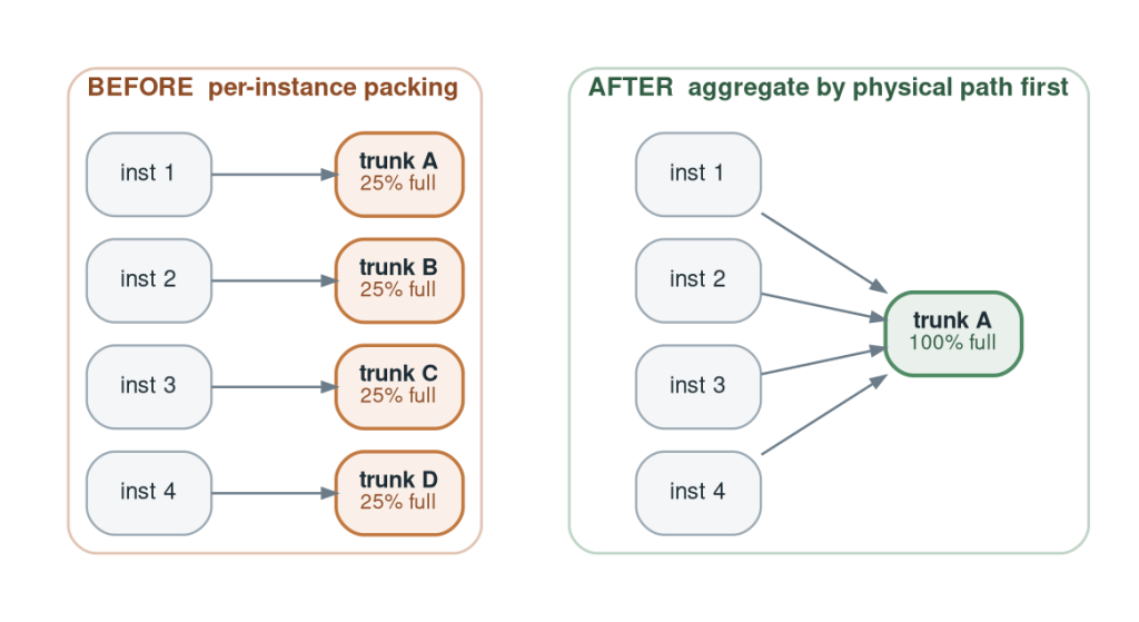
A single AI region has thousands of rack pairs, so direct cabling between every pair is infeasible. Aggregation is the structural response: for rack pairs crossing the same rooms, the module rolls up their strand demand, hands it to a shared aggregation rack, runs a few large trunks, and fans out at the far end. This happens per physical (source-rack, destination-rack) path, not per schematic instance. A high-density trunk is a shared bundle, and sizing must treat every instance on it as one cable, or the BOM undercounts (Figure 6).
Path diversity layers on top: where failure tolerance is required, the logic splits strands across multiple aggregation racks, conduits, and campus routes. It is resource intensive, so it is applied selectively.
Cable products at the topology level
Aggregation reduces cable count, not complexity. The module chains a small menu of products, each enabling a different rack-to-rack pattern.
- Patch cord. Two strands, one cable per link; used at channel ends.
- High-density (HD) connectors. MTP/MPO 12- or 24-fiber connectors packing many strands per cable; they carry most aggregated traffic.
- Fan in/out. An HD connector broken out into lower-density connectors, serving multiple destinations from one aggregated cable.
- Shuffle. HD connectors on both ends with a permuted strand map, interconnecting racks in a crossbar.
Strand-level circuit identity
Once fiber passes through a breakout and a cassette, “which circuit owns this strand?” stops being answerable from the cable graph alone (e.g., a 24-strand trunk carries strands from a dozen circuits, interleaved). The engine tags every strand at every connector on every cable with the circuit it belongs to, composing the tag through each connector’s internal strand mapping. Without this, end-to-end light-path validation fails on every channel (Figure 7).
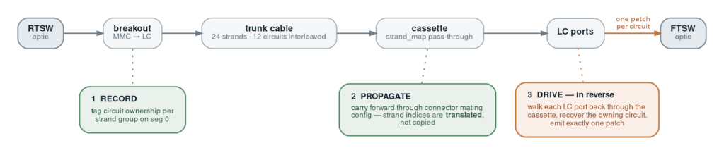
Figure 7. Recording and propagating strand-level circuit ownership.
Proving fiber correctness: light-path tracing as ground truth
A generator cannot certify itself. An independent tracer walks the built plant end to end—device optic through every cable, connector, and cassette to the destination optic—reconstructing every channel.
| Validation | Rule |
|---|---|
| Connectivity | every LNTG circuit has a physical light path |
| Polarity | every TX/RX strand pairing must land on the correct receiving position at the far end |
| Channel loss | total estimated optical loss along the channel is within the tolerance budget |
| Product compatibility | connector, fiber-adapter panel, cassette, and optic mating are all allowable at every junction |
| LNTG device | naming, elevation, and every topology device accounted for in the design |
Because the tracer walks the built model, its results are ground truth for what the engine produced, not what the schematic intended—divergence shows up before a cable is ordered.
Output and coverage
The design is a fully materialised model in which every cable, connector, and panel port is a first-class object. From it the engine emits a procurement-ready bill of materials and rack-by-rack installation instructions; because those come from the model the tracer validates, they cannot drift. The engine covers roughly 70% of fiber design projects today and has produced the first fully automated, end-to-end design for a new region.
Next steps and open problems
- End-to-end traceability. Each stage validates its own output today. What is missing is one chain of custody from logical intent to an ordered cable line item, so late changes propagate forward automatically.
- New infrastructure constraints: enhancing power and cooling models. Planogram today treats power as a fixed per row budget, simplified from reality. To improve this, we will be improving our modeling of power and cooling fungibility, including vale-train and bus bar placements on our floorplans .
- Brownfield designs. Everything here assumes a greenfield floor plan. Complex migrations, where installed equipment and existing fiber constrain what may move, is to be supported in the future.
Additional resources:
- Check out our SIGCOMM ’26 paper for more on the optimization model.

